Week 4 (cont.)#
Lecturer: Pritam Bhattacharya, BITS Pilani, Goa Campus
Date: 22/Aug/2021
Topics Covered#
- Rules to Find Big\(\mathcal{O}\) Notation (cont.)
- Little\(\mathcal{o}\) and Little\(\omega\)
- Bubble Sort
- Sort Function
- Optimized Sort Function
- Algorithm Analysis
- Time Complexity
- Space Complexity
Rules to Find Big\(\mathcal{O}\) Notation (cont.)#
- It is considered poor taste to include constant factors and lower order terms in the big\(\mathcal{O}\) notation
- Consider a function \(2n^2\) is \(\mathcal{O}(4n^2 + 6nlog(n))\), although this is right it is always easier and simpler to write \(\mathcal{O}(n^2)\)
| Logrithmic | Linear | Quadractic | Polynomial | Exponential |
|---|---|---|---|---|
| \(\mathcal{O}(log(n))\) | \(\mathcal{O}(n)\) | \(\mathcal{O}(n^2)\) | \(\mathcal{O}(n^k)\ (k \ge 1)\) | \(\mathcal{O}(a^n)\ (a \gt 1)\) |
- Even though in general we ignore constants in the big\(\mathcal{O}\) notation, we need to be careful and check if the constants have very large constants, in this case big\(\mathcal{O}\) might not be the right assumption for an algorithm.
| Some Functions Ordered By Growth Rate | Commone Name |
|---|---|
| \(\mathcal{O}(log(n))\) | Logrithmic |
| \(\mathcal{O}(log^2(n))\) | Polytlogrithmic |
| \(\mathcal{O}(\sqrt{n})\) | Square Root |
| \(\mathcal{O}(n)\) | Linear |
| \(\mathcal{O}(nlog(n))\) | Linearithmic |
| \(\mathcal{O}(n^2)\) | Quadratic |
| \(\mathcal{O}(n^3)\) | Cubic |
| \(\mathcal{O}(2^n)\) | Exponential |
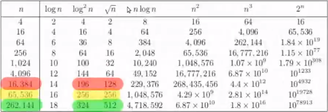
- In the above chart you see that \(\sqrt{n}\) crosses over much later over \(log^2(n)\) in comparison to other function pairs.
Little\(\mathcal{o}\) and Little\(\omega\)#
No matter what value of \(c \gt 0\) we choose, we need to see if \(g(n) \ge f(n)\). For example for a functions \(12n^2 + 6n\), the little\(\mathcal{o}\) is \(\mathcal{o}(n^3)\).
if \(f(n)\) is \(\mathcal{o}(g(n)\) then \(g(n)\) is \(\omega(f(n))\)
Bubble Sort#
Sort Function#
BubbleSort(int [] A, int n)
    Input: An array A containing n>= 1 integers
    Output: The sorted version of the array A

    for i = 0 to (n - 1)
        for j = 0 to (n - 1 - i)
            if A[i] > A[j + 1]
                # swap A[j] with A[j + 1]
                A[j] <-> A[j + 1]
    return A
Optimized Sort Function#
BubbleSortOptimized(int [] A, int n)
    Input: An array A containing n>= 1 integers
    Output: The sorted version of the array A

    for i = 0 to (n - 1)
        swaps = 0
        for j = 1 to (n - 1 - i)
            if A[i] > A[j + 1]
                # swap A[j] with A[j + 1]
                A[j] <-> A[j + 1]
                swaps <- swaps + 1
            if swaps == 0
                break
    return A
Algorithm Analysis#
Time Complexity#
In the basic sort function, for every value of \(i\), the inner loop indexed by \(j\) is done upto \(n - 1\) number of times and the outer loop indexed by \(i\) also runs \(n - 1\) times as well.
So the worst case time complexity is \(\mathcal{O}((n - 1)(n - 1)) = \mathcal{O}(n^2)\)
Best case time complexity (Where array is already sorted) is also \(\mathcal{O}(n^2)\)
Now taking the optimized sort function, we see that at the worst case the function behaves exactly like the basic sort function so the worst case time complexity is still \(\mathcal{O}(n^2)\), but in the best case the outer loop will run only once, so the best case time complexity is \(\mathcal{O}(n)\) since only the inner loop will run completely once.
Space Complexity#
Since no extra data structures were used, the space used is constant, so the space complexity in all cases is \(\mathcal{O}(1)\)