Week 2#
Lecturer: G Venkiteswaran, Faculty for BITS Pilani
Date: 01/Aug/2021
Topics Covered#
- Vector Norms
- Common Norms
- Equivalence of Norms
- Matrix Norms
- Solution of Linear systems
- Gauss elimination methods
- Pitfalls of Gauss Elimination Algorithms
- Division By Zero
- Round-off Errors
- Operations Count for Gaussian Elimination
- Pitfalls of Gauss Elimination Algorithms
- Ill Conditioned Systems
- Condition Number
Vector Norms#
A function \(|| . || : R^n \rightarrow R\) is a vector norm if it has the following properties:
1. \(||x|| \ge 0\) for any vector \(x \in R^n\), and \(||x|| = 0\) if and only if \(x = 0\).
2. \(||\alpha x|| = |\alpha|\ ||x||\) for any vector \(x \in R^n\), and any scalar \(\alpha \in R\).
3. \(||x+y|| \le ||x|| + ||y||\) for any vectors \(x,\ y \in R^n\). This property is called the triangle inequality (Sum of two sides is greater than the third)
4. Also to be noted is if the dimension value \(n=1\) then the modulus value function (\(|x|\)) is a vector norm. (where mod function is \(|x| = \max(x,-x)\))
Common Norms#
The most commonly used vector norm is belong to the family of \(l_p\) norms, which are defined by:
The following \(l_p\) norms are more used than others:
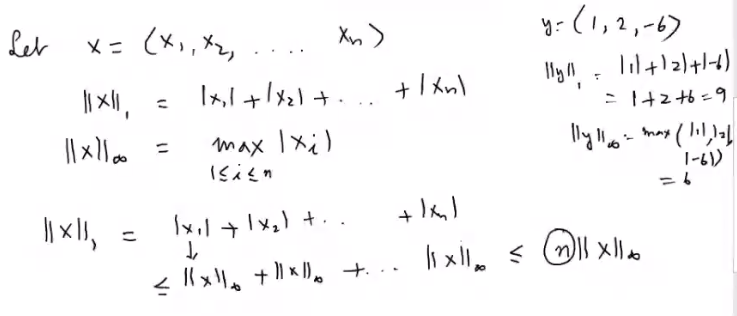
1. \(p=1:\ The\ l_1\ norm\ ||x||_1 = |x_1| + |x_2| + \dots + |x_n|\)
2. \(p=2:\ The\ l_2\ norm\ or\ Euclidean\ norm ||x||_2 = \sqrt{x_1^2 + x_2^2 + \dots + x_n^2} = \sqrt{x^Tx}\)
3. \(p=1:\ The\ l_\infty\ norm\ ||x||_{\infty} = \max_{1\le i\le n}|x_i|\)
Equivalence of Norms#
We say that two vector norms are equivalent if there exists constants \(C_1\) and \(C_2\), that are independent of \(x\), such that for any vector \(x \in R^n\)
Remember that the above equation does not show any relation between \(C_1\) or \(C_2\) or \(\alpha\) or \(\beta\)
Consider the above example, we take the two forms of \(l_p\) norms, the \(l_1\) and the \(l_\infty\).
You can see that each term of \(||x||_1\) is \(\le \ ||x||_\infty\) hence we can say that the total sum \(||x||_1 \le n||x||_\infty\).
This shows the equivalence of \(l_1\) and \(l_\infty\) norm.
Matrix Norms#
Some commonly used matrix norms are:
1. Matrix norm corresponding to vector \(1\)-norm is maximum modulus/absolute column sum:
You can see that we take the maximum of the absolute sum of the columns
- Matrix norm corresponding to vector \(\infty\)-norm is maximum modulus/absolute column sum:
You can see that we take the maximum of the absolute sum of the columns
- Matrix norm corresponding to vector \(2\)-norm is given as:
Question asked: What is the significance of a norm for a matrix?
Visualizing the above through Octave commands:
>> A = [2,1,1;3,2,1;-2,0,1]
A =

   2   1   1
   3   2   1
  -2   0   1

>> norm(A, 1)
ans = 7
>> norm(A, 'inf')
ans = 6
>> norm(A, 'fro')
ans = 5
>> norm(A, 2)
ans = 4.6758
Question to ask: if \(||A||_2 = |A||_F\) why are the results different in the above octave result?
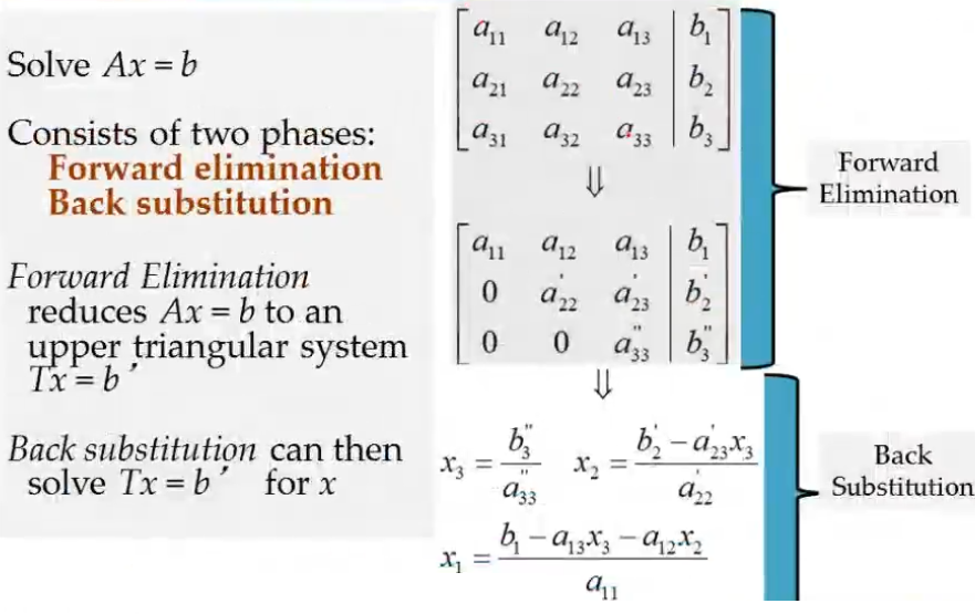
Solution of Linear systems#
Matrix form of Linear Systems
We can take m linear equations and write them as a single Vector equation like
- Where coefficient matrix \(A = [a_{jk}]\) is the \(m\ x\ n\) matrix
- Where all the variables are in the vector \(x = [x_k]\) with size \(n\ x\ 1\)
- Where all the constants are in vector b \(b = [b_j]\) with size \(m\ x\ 1\)
Gauss Elimination#
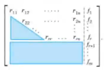
Consider the above image, at the end of gauss elimination, the row echelon form would hold a rank say \(r\), then we can say:
1. The matrix is a upper triangular form
2. The first \(r\) rows are non zero
3. Exactly \(m-r\) rows would be zero rows
4. The rhs can have two possibilities:
1. The rhs has exactly \(m-r\) zero rows: This means there is atleast one solution for the linear system of equations
2. The rhs has less than \(m-r\) zero rows: This means the equations are inconsistent
5. If the system is consistent and the \(r = n\) then there is exactly one solution
6. In case of infinitely many solutions, take arbiterary values for \(x_{r+1},\dots x_n\), then solve the \(r\)th equation for \(x_r\), then the \((r-1)\)st equaation for \(x_{r-1}\), and so on up the line till the solutions are found
7. The complexity for calculating this is \(O(n^3)\), where \(n\) is the number of rows
Pitfalls of Gauss Elimination Algorithms#
Division By Zero#
It is possible that in the above considered example, the denominator can end up being a zero value. For example consider the example below:
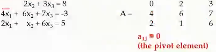
Here the coefficient of \(x_1\) in the first equation is 0, hence to avoid the above issue we can interchange rows \(R_1 \rightarrow R_2\). This is called pivoting and that will make it easier to bring about the REF form for the matrix.
Round-off Errors#
- Because computers can carry limited number of significant figures, round off errors will occur and they will propagate for every iteration.
- This problem becomes very apparent when the number of equations become very large.
- To avoid this one must use double-precision numbers. Albeit it being slow, the result will be more correct
Operations Count for Gaussian Elimination#
The details for the operation counts for several operations done is explained in the page here: GaussianEliminationPython#Operations Count
Ill Conditioned Systems#
Consider the following system of linear equations:
\(x_1 + 2x_2 = 10\)
\(1.1x_1 + 2x_2 = 10.4\)
We get the values of \(x_1 = 4.0\) and \(x_2 = 3.0\)
If let us say that when someone modeled this equation they had made a miscalculation leading to changing one of the coefficients of \(x_1\) from \(1.1\) to \(1.05\) making the above system of equations as follows:
\(x_1 + 2x_2 = 10\)
\(1.05x_1 + 2x_2 = 10.4\)
We get the values of \(x_1 = 8.0\) and \(x_2 = 1.0\)
From the above two results you can see that there is a big variance in the results when there is a small change in the coefficients, such system of equations are said to be ill conditioned
Condition Number#
The condition number is a metric that is used to see if a system of equations is ill informed or not. Condition number of a non singular matrix A is defined as:
By convention \(\kappa(A) = \infty\) if \(A\) is singular (A matrix whose determinant is 0, and hence has no inverse)
Example:
- Once conditions are calculated, we can say that whenever the condition number is in the range of 4 to 5 then they are well informed but if the condition is around a 100 or so then they are more ill conditioned in nature.
- There is no clear distinction between well informed and ill informed system of equations