Week 6 (cont.)#
Lecturer: G Venkiteswaran, Faculty for BITS Pilani
Date: 7/Sep/2021
Topics Covered#
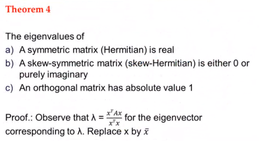
Special Matrices#
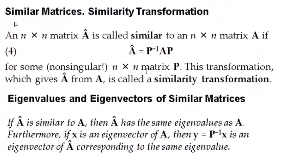
Similarity Of Matrices#
>> A = rand(4, 4)
A =

   5.8181e-01   9.6943e-01   4.2533e-01   6.4573e-01
   5.4844e-01   3.2016e-01   9.8479e-01   7.1938e-02
   9.0286e-01   8.2269e-01   6.9796e-02   2.7225e-01
   3.1388e-01   6.8389e-03   1.9440e-01   5.5537e-01

>> eig(A)
ans =

   2.0028 +      0i
  -0.5037 + 0.2040i
  -0.5037 - 0.2040i
   0.5318 +      0i

>> P = [6, 10, 11, 2; 2, 3, 5, 6; 19. 21. 61, 63; 39, 37, 79, 83]
P =

    6   10   11    2
    2    3    5    6
   19   21   61   63
   39   37   79   83

>> det(P)
ans = 1.1352e+04
>> B = inv(P) * A * P
B =

  -13.8730  -16.5433  -39.9569  -38.2545
   19.8346   23.1043   56.8459   55.2196
   -7.9618   -9.4378  -25.1538  -24.5634
    5.5832    6.7917   18.0890   17.4496

>> eig(B)
ans =

   2.0028 +      0i
   0.5318 +      0i
  -0.5037 + 0.2040i
  -0.5037 - 0.2040i
We see that \(A\) and \(B\) both share the same Eigen values, so \(A\) and \(B\) are similar matrices
So for a random matrix \(P\), we can find a similar matrix for \(A\) by doing:
\(B = P^{-1} . A . P\)
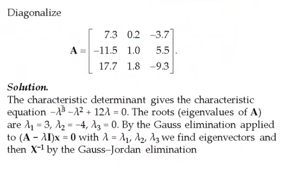
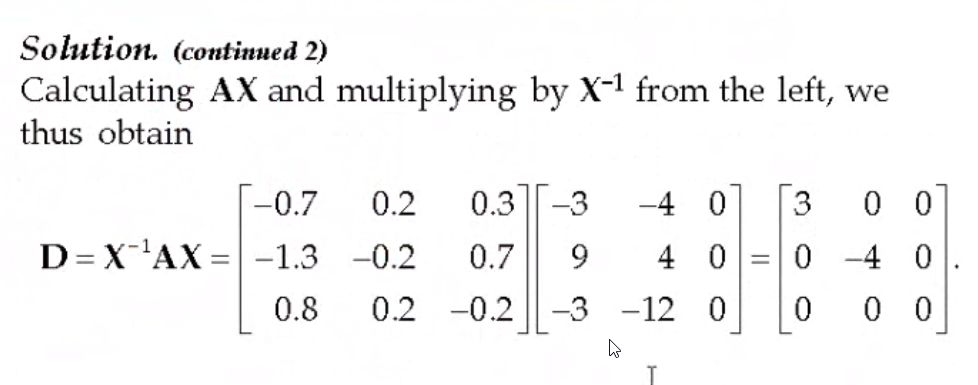
Diagonalization#
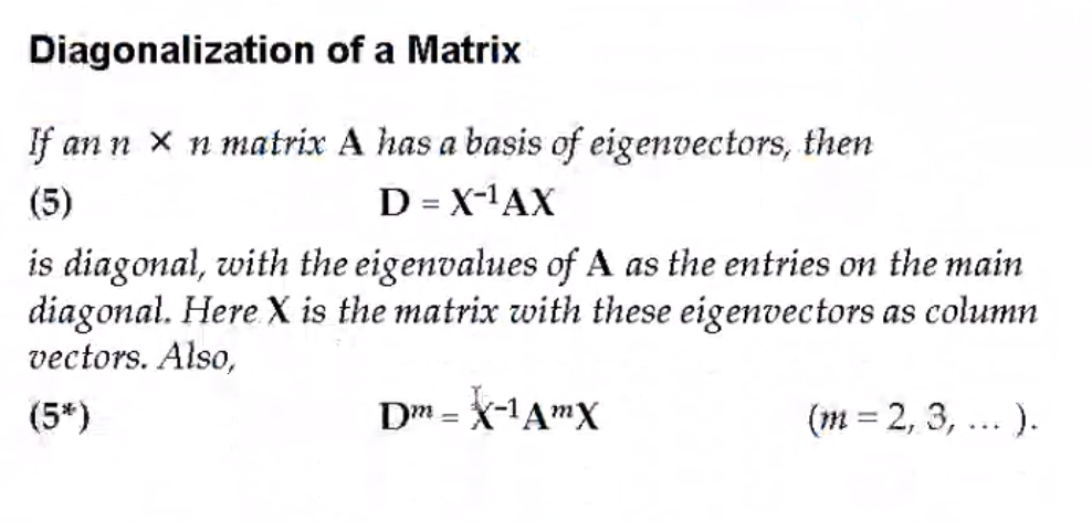
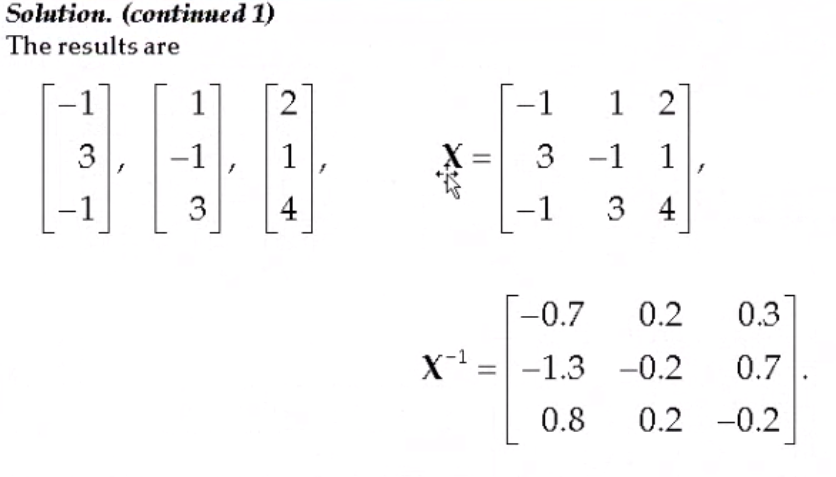
These 3 vectors are independent so,
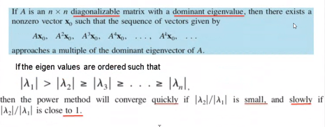
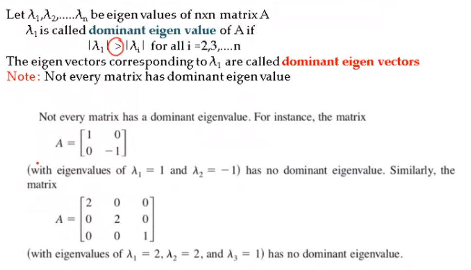
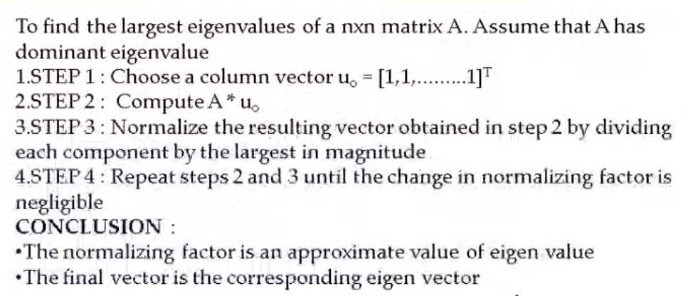
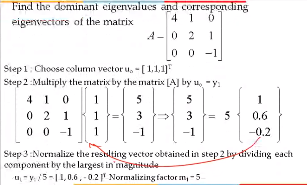
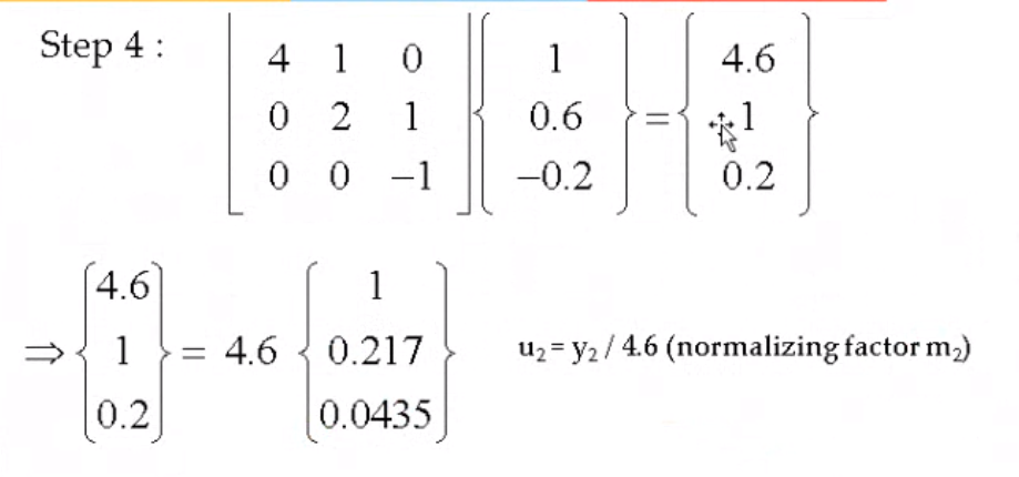
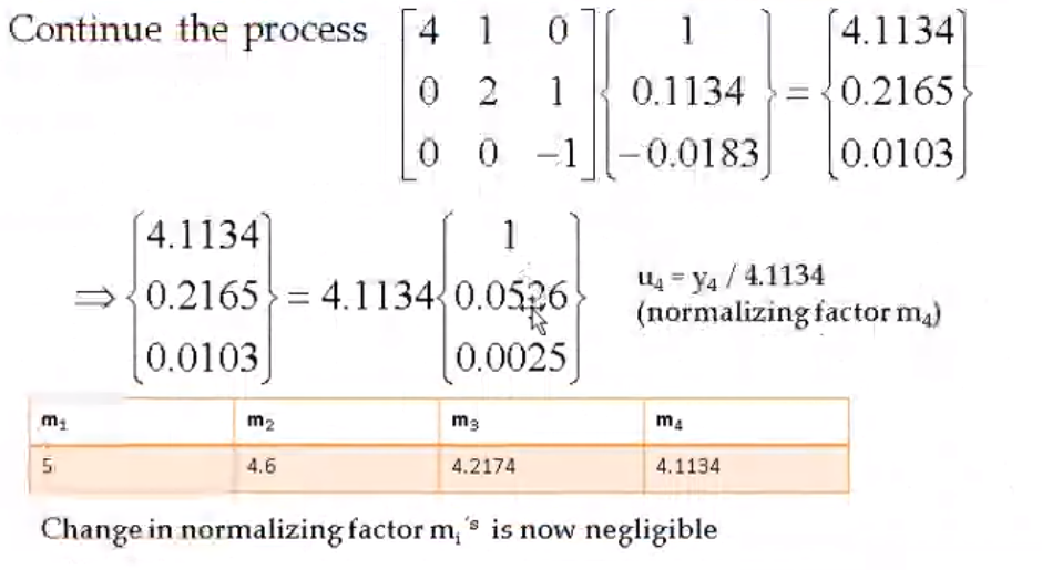
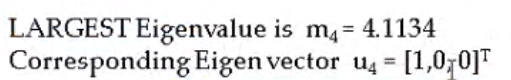
Dominant Eigen Value#
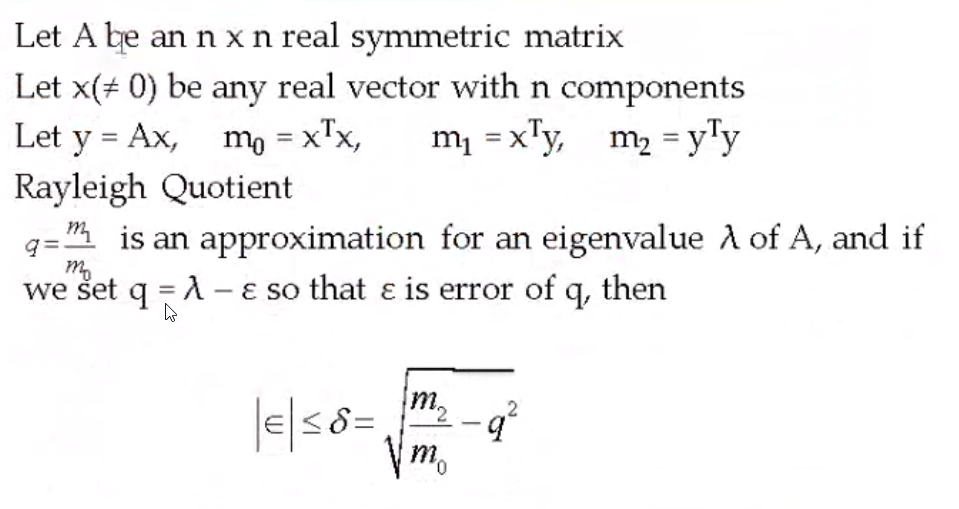
Rayleigh's Quotient#
Go through the excel sheet
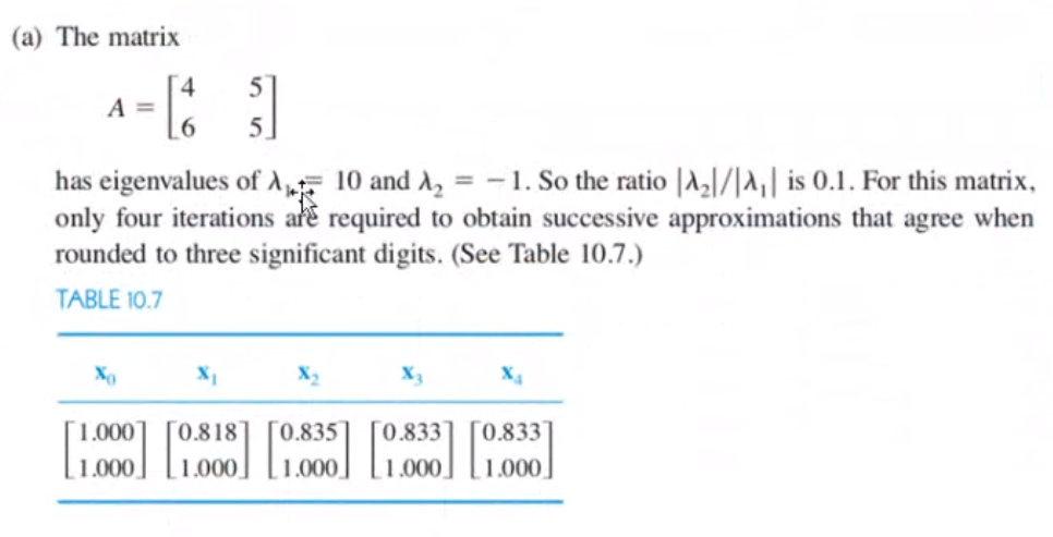
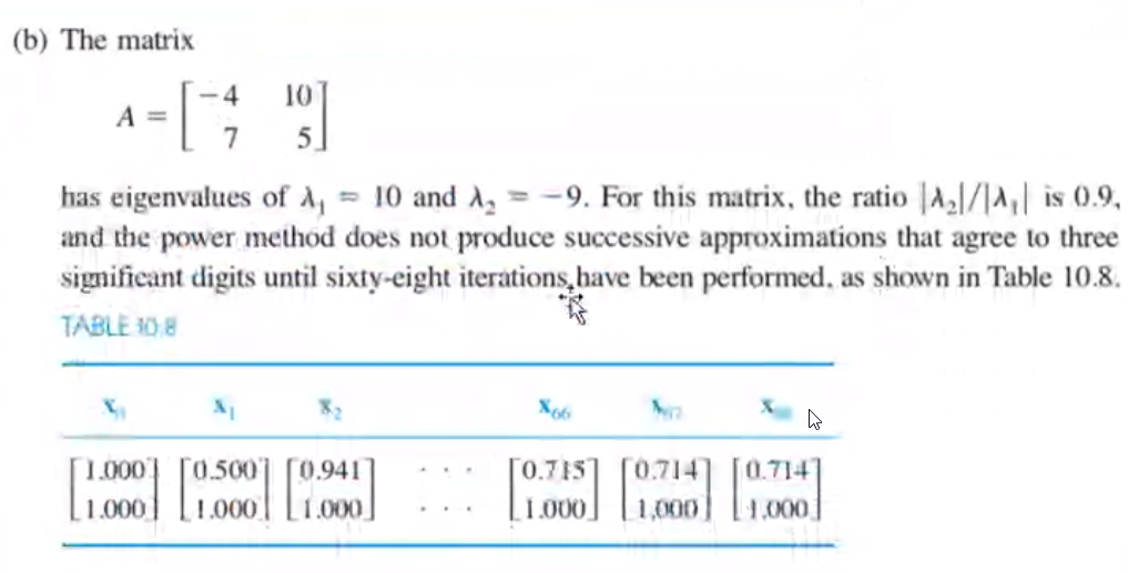
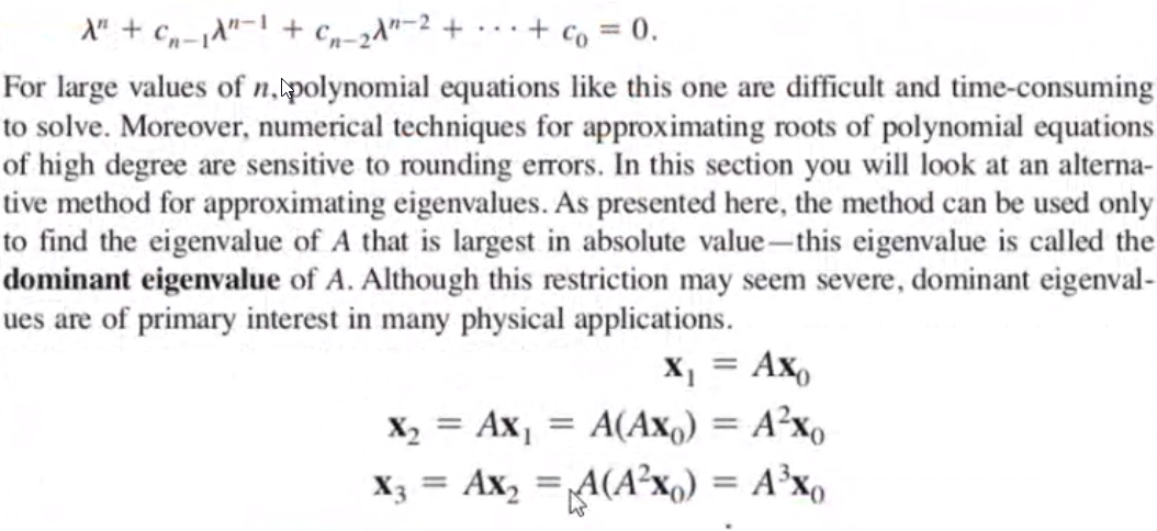
Power Method for#
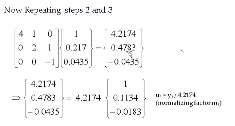
Convergence of Power Method#