Week 4 (cont.)#
Lecturer: Barsha Mitra, BITS Pilani, Hyderabad Campus
Date: 22/Aug/2021
Topics Covered#
- Terminology and Basic Algorithms
- Notations and Definitions
- Synchronous Single-Initiator Spanning Tree Algorithm using Flooding
- Algorithm Design
- Struct for each process \(P_i\)
- Algorithm pseudo code
- Algorithm in action
- Algorithm Design
- Broadcast and Convergecast Algorithm on a Tree
- Broadcast Algorithm
- Convergecast Algorithm
- Complexity
- Message Ordering
Terminology and Basic Algorithms#
Notations and Definitions#
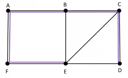
- Undirected unweighted graph \(G = (M, L)\), represents topology of an example graph such as the one shown below:
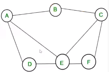
- Vertices are nodes
- Edges are channels
- \(n = |N|\), Cardinality of set of all nodes \(N = [A, B, C, D, E, F]\)
- \(l = |L|\), Cardinality of set of all edges \(L = [AB, BC, CF, DE, EF, AD, AE, CE]\)
- diameter of a graph :
- minimum number of edges that need to be traversed to go from any node to any other node
- \(Diameter = max_{i, j \in N}\), Length of the shortest path between i and j where j belongs to the set N. We basically find all the minimum distances from i to all j and the diameter is the maximum value
- In the above example let \(i = A\) and \(j = [A, B, C, D, E, F]\) then we can say that the max value of the lengths is 2 (In case of the path length for A to F), so the \(diameter = 2\)
- A spanning tree is a tree where the graph does not have any edges that will cause cycles in it. An example for a spanning tree for the above example is shown below:
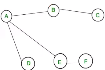
- As a rule of thumb, a spanning tree for a graph with \(n\) nodes, will have \(n - 1\) edges
- So in the example graph has 6 nodes and the number of edges in the spanning tree is 5.
Synchronous Single-Initiator Spanning Tree Algorithm using Flooding#
- Algorithm executes steps synchronously (When a message is sent, the sender waits till all the other nodes receives the messages)
- Root of the graph initiates the algorithm (An arbitrary node can be selected as the root)
- QUERY messages are flooded. This means that first the root node will send a message to all its nearby nodes, and inturn those nodes will send it to its neighbors and so on.
- The final spanning tree will have the root node as the initial arbitrary node selected in the graph.
- Each process \(P_i (P_i \ne root)\) should output its own parent for the spanning tree. In distributed computing we interchangeably use nodes and processes
Algorithm Design#
Struct for each process \(P_i\)#
| Variables maintained at each \(P_i\) | Initial variable values at each \(P_i\) |
|---|---|
| int visited | 0 |
| int depth | 0 |
| int parent | NULL |
| set of int Neighbors | set of neighbors |
Algorithm pseudo code#
Algorithm for Pi

When Round r = 1
if Pi = root then
    visited = 1
    depth = 0
    send QUERY to Neighbors
if Pi receives a QUERY message then
    visited = 1
    depth = r
    parent = root
    plan to send QUERY to Neighbors at the next round

When Round r > 1 and r <= diameter
if Pi planned to send in previous round then
    Pi sends QUERY to Neighbors
if Pi receives QUERY messages then
    visited = 1
    depth = r
    parent = any randomly selected nodes from which Query was receives plan to send QUERY to Neighbors but not to any nodes from which send was received
Algorithm in action#
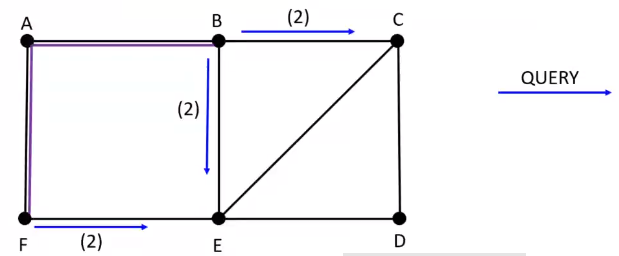
Round 1 :
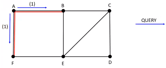
Root \(A\) sends \(QUERY\) to neighbors \([B, F]\)
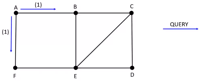
\(B\) and \(F\) set \(A\) as parent and plans to send \(QUERY\) to its neighbors
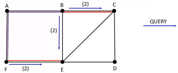
Round 2 :
\(B\) sends \(QUERY\) to neighbors \([C, E]\) and \(F\) sends \(QUERY\) to neighbors \([E]\)
\(E\) randomly chooses \(F\) as parent and \(C\) chooses \(B\) as parent and both \(E\) and \(F\) plans to send \(QUERY\) to its neighbors
Round 3 :
\(E\) sends \(QUERY\) to neighbors \([C, D]\) and \(C\) sends \(QUERY\) to neighbors \([E, D]\)
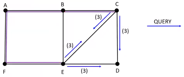
Since \(C\) and \(E\) are already visited, the \(QUERY\) is ignored in those cases and \(D\) randomly chooses \(C\) as parent over \(E\)
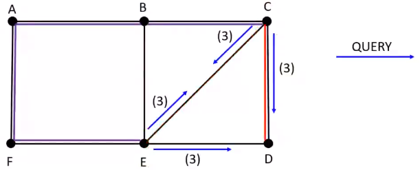
The spanning tree generated is as follows :
The above spanning tree has 6 nodes and 5 edges
Broadcast and Convergecast Algorithm on a Tree#
A spanning tree is useful for distributing (via Broadcast) and collecting information (via Convergecast) to and from all the nodes
Broadcast Algorithm#
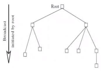
- BC1:
- The root sends the information to be sent to all its children
- BC2:
- When a non root node receives information from its parent, it copies it and forwards it to its children
Convergecast Algorithm#
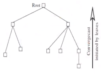
- CVC1:
- Leaf node sends what it needs to report to its parent
- CVC2:
- At a non leaf node that is not root, a report is received from all the child nodes, the collective report is sent to its parent
- CVC3:
- When a root node receives information from its child nodes, the global function is evaluated using the reports
Complexity#
- Each broadcast and each convergecast requires \(n - 1\) messages.
- Each broadcast and each convergecast requires time equal to the maximum height \(h\) of the tree which is \(\mathcal{O}(n)\)
Message Ordering#
Group Communication#
- Broadcast - Sending a message to all members in the distributed system
- Multicasting - A message is sent to a certain subset, identified as a group, of the processes in the system.
- Unicasting - Point-to-point message communication
Causal Order#
- Causal Order is explained here: Week3DC#Causal Ordering Model
- 2 criteria must be satisfied by causal ordering protocol
- Safety:
- A message M arriving at a process may need to be buffered until all system wide messages sent in the causal past of the send(M) event to the same destination have already arrived
- Distinction is made between:
- Arrival of messages at a process
- Event at which the message is given to the application process
- Liveness:
- A message that arrives at a process must be eventually be delivered to the process
- Safety:
Raynal-Schiper-Toueg Algorithm#
- Each message M should carry a log of
- All other messages
- Send causally before M's send event, and sent to the same destination dest(M)
- Log can be examined to ensure when it is safe to deliver a message
- Channels are assumed to be FIFO
Local Variables#
- array of int \(SENT[1 .... n, 1 .... n]\) (n x n array)
- Where \(SENT_i[j, k]\) = no. of messages sent by \(P_j\) to \(P_k\) as known to \(P_i\)
- array of int \(DELIV[1 .... n]\)
- Where \(DELIV_i[j]\) = no. of messages from \(P_j\) that have been delivered to \(P_i\)
The Algorithm#
- Message Send Event, where \(P_i\) wants to send message \(M\) to \(P_j\):
- \(send(M, SENT)\) to \(P_j\) (Here \(SENT\) array is the log which will be used to determine if the message needs to be buffered or not)
- \(SENT[i, j] = SENT[i, j] + 1\)
- Message Arrival Event, when \((M, SENT_j)\) arrives at \(P_i\) from \(P_j\):
- deliver \(M\) to \(P_i\) when for each process \(x\),
- \(DELIV_i[x] \ge SENT_j[x, i]\)
- \(\forall x, y, SENT_i[x, y] = max(SENT_i[x, y], SENT_j[x, y])\)
- \(DELIV_i[j] = DELIV_i[j] + 1\)
Algorithm Complexity#
- Space complexity at each process: \(\mathcal{O}(n^2)\) integers
- Space overhead per message: \(n^2\) integers
- Time complexity at each process for each send and deliver event: \(\mathcal{O}(n^2)\)
Algorithm in action#
Assume following steps have occurred till now
- \(P_1\) sent 3 messages to \(P_2\)
- \(P_1\) sent 4 messages to \(P_3\)
- \(P_2\) sent 5 messages to \(P_1\)
- \(P_2\) sent 2 messages to \(P_3\)
- \(P_3\) sent 4 messages to \(P_2\)
Variable state
Assuming \(SENT\) of all \(P\) is aware of all the other values of \(SENT\), \(SENT\) of \(P_1\):
| 0   | 3   | 4   |
| 5   | 0   | 2   |
| 0   | 4   | 0   |
Assume the following values for \(DELIV\) arrays
\(DELIV_1 = [0, 4, 0]\)
\(DELIV_2 = [3, 0, 4]\)
\(DELIV_3 = [3, 2, 0]\)
MESSAGE EVENTS:
Now if, \(P_1\) sends \(m_1\) to \(P_2\)
1. \(SEND\) event from \(P_1\)
1. \(SENT_1\)
| 0   | 3   | 4   |
| 5   | 0   | 2   |
| 0   | 4   | 0   |
2. Send \((m_1, SENT_1)\)
3. Updated \(SENT_1\)
| 0   | 3+1 | 4   |    | 0   | 4   | 4   |
| 5   | 0   | 2   | => | 5   | 0   | 2   |
| 0   | 4   | 0   |    | 0   | 4   | 0   |
2. \(RECEIVE\) \(m_1\) from \(P_1\) at \(P_2\)
1. \(DELIV_2[1] \ge SENT_1[1, 2]\)
2. \(DELIV_2[3] \ge SENT_1[3, 2]\)
3. Deliver \(m_1\) to \(P_2\)
4. \(DELIV_2[1] = DELIV_2[1] + 1 = 4\)
5. \(DELIV_2 = [4, 0, 4]\)
6. \(SENT_2\)
| 0   | 3   | 4   |
| 5   | 0   | 2   |
| 0   | 4   | 0   |
Now if, \(P_3\) sends \(m_2\) to \(P_2\)
1. \(SEND\) event from \(P_3\)
1. \(SENT_3\)
| 0   | 3   | 4   |
| 5   | 0   | 2   |
| 0   | 4   | 0   |
2. Send \((m_2, SENT_3)\)
3. Updated \(SENT_3\)
| 0   | 3   | 4   |    | 0   | 3   | 4   |
| 5   | 0   | 2   | => | 5   | 0   | 2   |
| 0   | 4+1 | 0   |    | 0   | 5   | 0   |
2. \(RECEIVE\) \(m_2\) from \(P_3\) at \(P_2\)
1. \(DELIV_2[1] \ge SENT_3[1, 2]\)
2. \(DELIV_2[3] \ge SENT_3[3, 2]\)
3. Deliver \(m_2\) to \(P_2\)
4. \(DELIV_2[3] = DELIV_2[3] + 1 = 5\)
5. \(DELIV_2 = [4, 0, 5]\)
6. \(SENT_2\)
| 0   | 3   | 4   |
| 5   | 0   | 2   |
| 0   | 4   | 0   |
Now if, \(P_1\) sends \(m_3\) to \(P_3\)
1. \(SEND\) event from \(P_1\)
1. \(SENT_1\)
| 0   | 4   | 4   |
| 5   | 0   | 2   |
| 0   | 4   | 0   |
2. Send \((m_2, SENT_3)\)
3. Updated \(SENT_3\)
| 0   | 4   | 4+1 |     | 0   | 4   | 5   |
| 5   | 0   | 2   | =>  | 5   | 0   | 2   |
| 0   | 4   | 0   |     | 0   | 5   | 0   |
2. \(RECEIVE\) \(m_3\) from \(P_1\) at \(P_3\)
1. \(DELIV_3[1] \ge SENT_1[1, 3]\) (FALSE)
2. \(DELIV_3[2] \ge SENT_1[2, 3]\) (TRUE)
3. Put \(m_3\) in buffer since the first condition failed, only process it after the other \(P_1\) messages are delivered to \(P_3\)