Week 6

Lecturer: Pritam Bhattacharya, BITS Pilani, Goa Campus

Date: 4/Sep/2021

Topics Covered

1. Merge Sort
   1. Steps
   2. Algorithm
      1. Merge Function
      2. Sort Function
   3. Algorithm Analysis
      1. Space Complexity
      2. Time Complexity

Merge Sort

Merge Sort is not an in-place sort like the other three that was explained above

Steps

Let us consider the following arrays
\(4, 1, 7, 5, 2, 3\)
Now let us split this array into two halves:
\(4, 1, 7\ |\ 5, 2, 3\)
And let us sort these two parts:
\(1, 4, 7\ |\ 2, 3, 5\)
When merging the above two parts, we maintain two pointers that start on either parts, and we compare the elements pointed by these two and place the smaller element into a new array and advance that pointer and repeat the above procedure till all the elements are compared.

Algorithm

Merge Function

merge(S1, S2, S):
    Input: Two arrays, S1, S2, of size n1 and n2 sorted in non decreasing order, and an empty array S of size n1 + n2
    Ouput: S, containing the elements from S1 and S2 in sorted order

    i <- 0
    j <- 0
    while i < n1 and j < n2 do
        if S1[i] <= S2[j] then
            S[i + j] <- S1[i]
            i <- i + 1
        else
            S[i + j] <- S2[j]
            j <- j + 1
    while i <= n1 do
        S[i + j] <- S1[i]
        i <- i + 1
    while i <= n2 do
        S[i + j] <- S2[j]
        j <- j + 1

Sort Function

The actual sorting is done in a divide and conquer fashion denoted by the below steps:
1. Divide: If \(S\) has zero or one element, return \(S\) immediately, it is already sorted, Otherwise put the elements of \(S\) into two sequences \(S_1\) and \(S_2\), each containing about half of the elements of \(S\)
2. Recur: Recursively sort the sequences \(S_1\) and \(S_2\)
3. Conquer: Put back the elements into S by merging the sorted sequences \(S_1\) and \(S_2\) into a sorted sequence.

sort(S):
    Input: An array of size n
    Ouput: The sorted version of the array S

    if n == 1 then
        return S
    if n == 2 then
        if S[0] > S[1] then
            S[0] <-> S[1]
        return S
    S1 <- {S[0], S[1], S[2], .... , S[n/2]}
    S1 <- {S[(n/2)+1], .... , S[n - 2], S[n - 1]}
    R1 <- sort(S1)
    R2 <- sort(S2)
    merge(R1, R2, R)         # R is an empty array of size n
    return R

Algorithm Analysis

Space Complexity

The recursive tree for a random input array would look something like this:

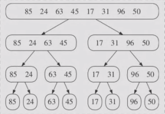
From the above image you can see that the number of memory blocks from the root to the leaf node of the recursive tree is at max \(n\), so:
Space Complexity: \(\mathcal{O}(n)\)

Time Complexity

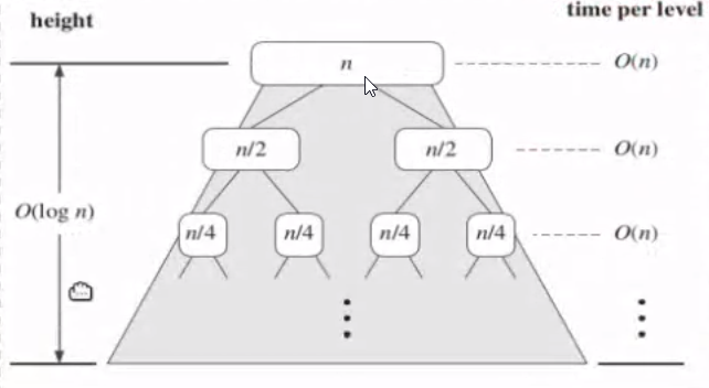
At every level, we do a total effort of merging in the order of \(\mathcal{O}(n)\)
The total height of the recursive tree is given by the order of \(\mathcal{O}(log\ n)\)
So Time Complexity: \(\mathcal{O}(n\ log\ n)\)

---

Tags: !DatastructuresAndAlgorithmsIndex