Notebook for data cleaning#
Data Cleaning: Data cleansing or data cleaning is the process of detecting and correcting (or removing) corrupt or inaccurate records from a record set, table, or database and refers to identifying incomplete, incorrect, inaccurate or irrelevant parts of the data and then replacing, modifying, or deleting the dirty or coarse data.
- Methods & techniques in Python on how to find and clean:
- Missing data
- Irregular data (outliers)
- Unnecessary data — repetitive data, duplicates, and more
- Inconsistent data — capitalization, data types, typos, addresses
Raw data is always messy, may suffer from various quality issues. We can't use it as it is. If you use such data for analysis, for example, feed into a machine learning model, you’ll get useless insights most of the time. That’s why data cleansing is a critical process for data analysts and data scientists.
- Useful Python Libraries
- pandas: a popular data analysis and manipulation tool, which will be used for most of our data cleaning techniques
- seaborn: statistical data visualization library
- Missingno Python library that provides a series of visualisations to understand the presence and distribution of missing data within a pandas dataframe.
- nltk: natural language toolkit
Case Study --> Russian housing market dataset
The goal of the project is to predict housing prices.
(30471, 292) There are 292 columns and 30471 rows in the data set
import pandas as pd df = pd.read_csv("sberbank-russian-housing-market/train/train.csv") df.head() df.shape# to check datatypes df.info()RangeIndex: 30471 entries, 0 to 30470 Columns: 292 entries, id to price_doc dtypes: float64(119), int64(157), object(16) memory usage: 67.9+ MB # to identify numeric and non-numeric attributes in the dataset numeric_cols = df.select_dtypes(include=['number']).columns non_numeric_cols = df.select_dtypes(exclude=['number']).columnsIndex(['id', 'full_sq', 'life_sq', 'floor', 'max_floor', 'material', 'build_year', 'num_room', 'kitch_sq', 'state', ... 'cafe_count_5000_price_2500', 'cafe_count_5000_price_4000', 'cafe_count_5000_price_high', 'big_church_count_5000', 'church_count_5000', 'mosque_count_5000', 'leisure_count_5000', 'sport_count_5000', 'market_count_5000', 'price_doc'], dtype='object', length=276)numeric_colsIndex(['timestamp', 'product_type', 'sub_area', 'culture_objects_top_25', 'thermal_power_plant_raion', 'incineration_raion', 'oil_chemistry_raion', 'radiation_raion', 'railroad_terminal_raion', 'big_market_raion', 'nuclear_reactor_raion', 'detention_facility_raion', 'water_1line', 'big_road1_1line', 'railroad_1line', 'ecology'], dtype='object') # Missing Datanon_numeric_cols- When data is missing for a column in a row. Ways to handle it:
- How to find out?
- Method #1: missing data (by columns) count & percentage
df[non_numeric_cols].info()RangeIndex: 30471 entries, 0 to 30470 Data columns (total 16 columns): # Column Non-Null Count Dtype --- ------ -------------- ----- 0 timestamp 30471 non-null object 1 product_type 30471 non-null object 2 sub_area 30471 non-null object 3 culture_objects_top_25 30471 non-null object 4 thermal_power_plant_raion 30471 non-null object 5 incineration_raion 30471 non-null object 6 oil_chemistry_raion 30471 non-null object 7 radiation_raion 30471 non-null object 8 railroad_terminal_raion 30471 non-null object 9 big_market_raion 30471 non-null object 10 nuclear_reactor_raion 30471 non-null object 11 detention_facility_raion 30471 non-null object 12 water_1line 30471 non-null object 13 big_road1_1line 30471 non-null object 14 railroad_1line 30471 non-null object 15 ecology 30471 non-null object dtypes: object(16) memory usage: 3.7+ MB all counts are same for non-numeric columns, hence no missing data id 0 timestamp 0 full_sq 0 life_sq 6383 floor 167 max_floor 9572 material 9572 build_year 13605 num_room 9572 kitch_sq 9572 dtype: int64num_missing = df.isna().sum() num_missing[:10]id 0.000000 timestamp 0.000000 full_sq 0.000000 life_sq 0.209478 floor 0.005481 max_floor 0.314135 material 0.314135 build_year 0.446490 num_room 0.314135 kitch_sq 0.314135 dtype: float64# to caclulate mean of missing values by columns num_missing = df.isna().mean() num_missing[:10]- Method #2: missing data (by columns) heatmap
# to visualise missing values
# heapmap can be created using "seaborn" and "missingno" libraries
import seaborn as sns

# since number of columns are very large, it would be difficult to visualise them at the same time. We can learn the patter
# pattern of missing data for the first 30 columns
cols= df.columns[:30]
colors = ["green", "blue"]
sns.heatmap(df[cols].isna(), cmap=sns.color_palette(colors))
![[Assets/DataVisualizationNotebook/output_19_1.png]] the column life_sq has missing values across different rows. While the column max_floor has most of its missing values # missingno The missingno library is a small toolset focused on missing data visualizations and utilities. So you can get the same missing data heatmap as above with shorter code. Requirement already satisfied: missingno in c:\users\bits-wilp\anaconda3\lib\site-packages (0.5.0) Requirement already satisfied: matplotlib in c:\users\bits-wilp\anaconda3\lib\site-packages (from missingno) (3.2.2) Requirement already satisfied: numpy in c:\users\bits-wilp\anaconda3\lib\site-packages (from missingno) (1.18.5) Requirement already satisfied: scipy in c:\users\bits-wilp\anaconda3\lib\site-packages (from missingno) (1.5.0) Requirement already satisfied: seaborn in c:\users\bits-wilp\anaconda3\lib\site-packages (from missingno) (0.10.1) Requirement already satisfied: kiwisolver>=1.0.1 in c:\users\bits-wilp\anaconda3\lib\site-packages (from matplotlib->missingno) (1.2.0) Requirement already satisfied: pyparsing!=2.0.4,!=2.1.2,!=2.1.6,>=2.0.1 in c:\users\bits-wilp\anaconda3\lib\site-packages (from matplotlib->missingno) (2.4.7) Requirement already satisfied: cycler>=0.10 in c:\users\bits-wilp\anaconda3\lib\site-packages (from matplotlib->missingno) (0.10.0) Requirement already satisfied: python-dateutil>=2.1 in c:\users\bits-wilp\anaconda3\lib\site-packages (from matplotlib->missingno) (2.8.1) Requirement already satisfied: pandas>=0.22.0 in c:\users\bits-wilp\anaconda3\lib\site-packages (from seaborn->missingno) (1.0.5) Requirement already satisfied: six in c:\users\bits-wilp\anaconda3\lib\site-packages (from cycler>=0.10->matplotlib->missingno) (1.15.0) Requirement already satisfied: pytz>=2017.2 in c:\users\bits-wilp\anaconda3\lib\site-packages (from pandas>=0.22.0->seaborn->missingno) (2020.1)!pip install missingno import missingno as msno msno.matrix(df.iloc[:, :30])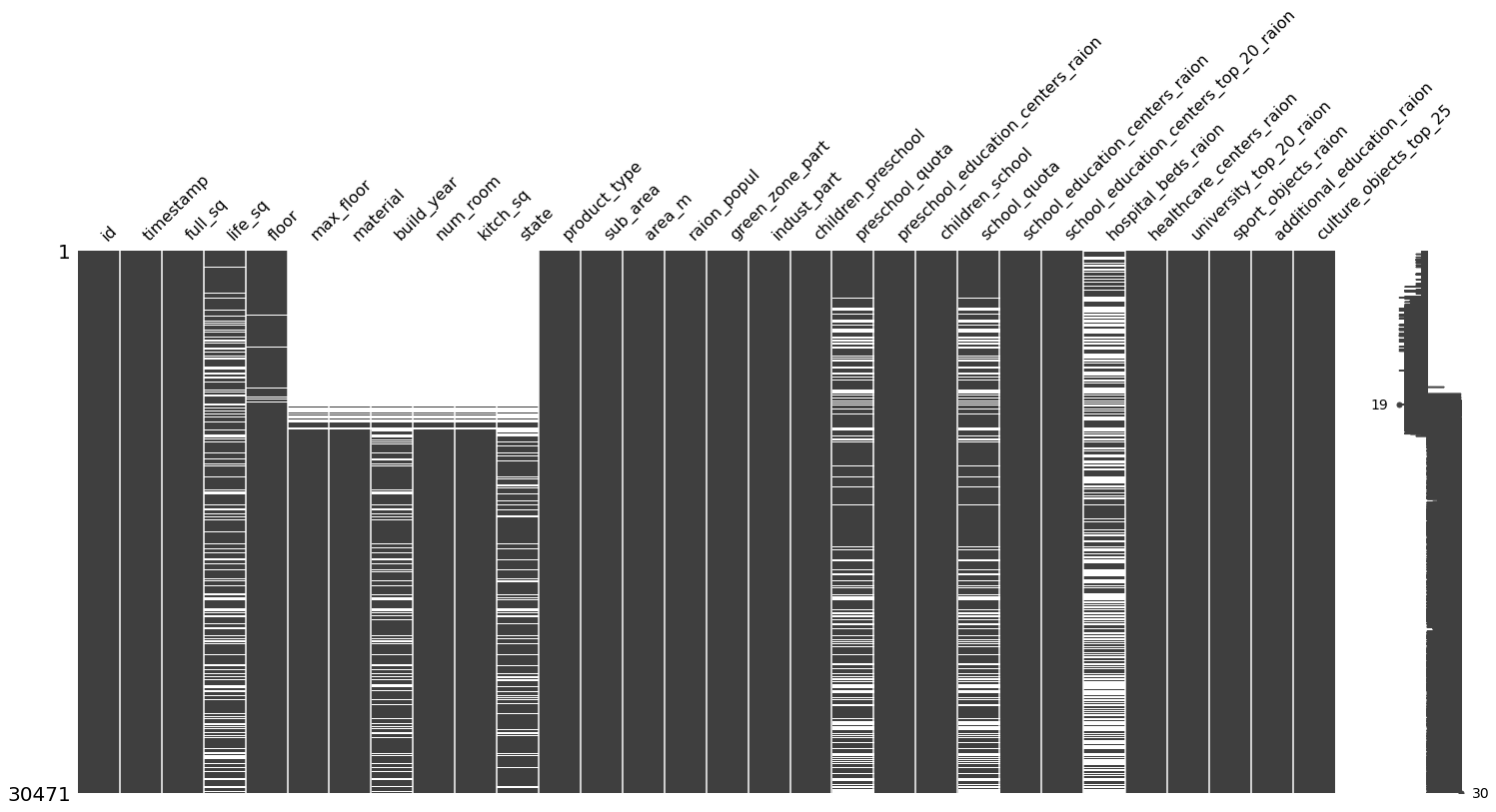 - Method #3: missing data (by rows) histogram
- summarize the missing data by rows.
missing_by_row = df.isna().sum(axis='columns')
missing_by_row.hist(bins=50)
![[Assets/DataVisualizationNotebook/output_24_1.png]] This histogram helps to identify the missing patterns among the 30,471 observations. For example, there are over 6,000 observations with no missing values, and close to 4,000 observations with 1 missing value. - How to handle missing data
- Methods:
- Technique #1: drop columns / features: drop the entire column or features with large number of missing values. But, this will cause a loss of information. Let’s consider the columns with a high percentage of missing.
max_floor 0.314135 material 0.314135 build_year 0.446490 num_room 0.314135 kitch_sq 0.314135 state 0.444980 hospital_beds_raion 0.473926 cafe_sum_500_min_price_avg 0.435857 cafe_sum_500_max_price_avg 0.435857 cafe_avg_price_500 0.435857 dtype: float64
num_missing[num_missing > 0.3]df.drop(['max_floor', 'material', 'build_year', 'num_room', 'kitch_sq','state','hospital_beds_raion', 'cafe_sum_500_min_price_avg','cafe_sum_500_max_price_avg', 'cafe_avg_price_500'],axis = 1) df.head()id timestamp full_sq life_sq floor max_floor material build_year num_room kitch_sq ... cafe_count_5000_price_2500 cafe_count_5000_price_4000 cafe_count_5000_price_high big_church_count_5000 church_count_5000 mosque_count_5000 leisure_count_5000 sport_count_5000 market_count_5000 price_doc 0 1 2011-08-20 43 27.0 4.0 NaN NaN NaN NaN NaN ... 9 4 0 13 22 1 0 52 4 5850000 1 2 2011-08-23 34 19.0 3.0 NaN NaN NaN NaN NaN ... 15 3 0 15 29 1 10 66 14 6000000 2 3 2011-08-27 43 29.0 2.0 NaN NaN NaN NaN NaN ... 10 3 0 11 27 0 4 67 10 5700000 3 4 2011-09-01 89 50.0 9.0 NaN NaN NaN NaN NaN ... 11 2 1 4 4 0 0 26 3 13100000 4 5 2011-09-05 77 77.0 4.0 NaN NaN NaN NaN NaN ... 319 108 17 135 236 2 91 195 14 16331452 5 rows × 292 columns
- Technique #2: drop rows / observations
df.dropna(axis=0, how='any', thresh=257, subset=None, inplace=True)
# thresh argument that specifies the number of non-missing values that should be present for each row in order not to be dropped.
df
id timestamp full_sq life_sq floor max_floor material build_year num_room kitch_sq ... cafe_count_5000_price_2500 cafe_count_5000_price_4000 cafe_count_5000_price_high big_church_count_5000 church_count_5000 mosque_count_5000 leisure_count_5000 sport_count_5000 market_count_5000 price_doc 0 1 2011-08-20 43 27.0 4.0 NaN NaN NaN NaN NaN ... 9 4 0 13 22 1 0 52 4 5850000 1 2 2011-08-23 34 19.0 3.0 NaN NaN NaN NaN NaN ... 15 3 0 15 29 1 10 66 14 6000000 2 3 2011-08-27 43 29.0 2.0 NaN NaN NaN NaN NaN ... 10 3 0 11 27 0 4 67 10 5700000 3 4 2011-09-01 89 50.0 9.0 NaN NaN NaN NaN NaN ... 11 2 1 4 4 0 0 26 3 13100000 4 5 2011-09-05 77 77.0 4.0 NaN NaN NaN NaN NaN ... 319 108 17 135 236 2 91 195 14 16331452 ... ... ... ... ... ... ... ... ... ... ... ... ... ... ... ... ... ... ... ... ... ... 30466 30469 2015-06-30 44 27.0 7.0 9.0 1.0 1975.0 2.0 6.0 ... 15 5 0 15 26 1 2 84 6 7400000 30467 30470 2015-06-30 86 59.0 3.0 9.0 2.0 1935.0 4.0 10.0 ... 313 128 24 98 182 1 82 171 15 25000000 30468 30471 2015-06-30 45 NaN 10.0 20.0 1.0 NaN 1.0 1.0 ... 1 1 0 2 12 0 1 11 1 6970959 30469 30472 2015-06-30 64 32.0 5.0 15.0 1.0 2003.0 2.0 11.0 ... 22 1 1 6 31 1 4 65 7 13500000 30470 30473 2015-06-30 43 28.0 1.0 9.0 1.0 1968.0 2.0 6.0 ... 5 2 0 7 16 0 9 54 10 5600000 29779 rows × 292 columns
- Technique #3: impute the missing with constant values.
df_copy = df.copy() numeric_cols = df_copy.select_dtypes(include=['number']).columns df_copy[numeric_cols] = df_copy[numeric_cols].fillna(-999) df_copy[non_numeric_cols] = df_copy[non_numeric_cols].fillna('_MISSING_') - Technique #4: impute the missing with statistics
#imputing numeric columns by median
med = df_copy[numeric_cols].median()
df_copy[numeric_cols] = df_copy[numeric_cols].fillna(med)
# imputing non-numeric columns by mode most_freq = df_copy[non_numeric_cols].mode() df_copy[non_numeric_cols] = df_copy[non_numeric_cols].fillna(most_freq)most_freqtimestamp product_type sub_area culture_objects_top_25 thermal_power_plant_raion incineration_raion oil_chemistry_raion radiation_raion railroad_terminal_raion big_market_raion nuclear_reactor_raion detention_facility_raion water_1line big_road1_1line railroad_1line ecology 0 2014-12-16 Investment Poselenie Sosenskoe no no no no no no no no no no no no poor id 0 timestamp 0 full_sq 0 life_sq 0 floor 0 .. mosque_count_5000 0 leisure_count_5000 0 sport_count_5000 0 market_count_5000 0 price_doc 0 Length: 292, dtype: int64 # Irregular data (outliers) Outliers could bias our data analysis results, providing a misleading representation of the data. Outliers could be real outliers or mistakes.#to check for missing values df_copy.isna().sum()- How to detect?
- Method #1: descriptive statistics
df_copy.describe()id full_sq life_sq floor max_floor material build_year num_room kitch_sq state ... big_church_count_5000 church_count_5000 mosque_count_5000 leisure_count_5000 sport_count_5000 market_count_5000 price_doc year month weekday count 2.977900e+04 2.977900e+04 2.977900e+04 2.977900e+04 2.977900e+04 2.977900e+04 2.977900e+04 2.977900e+04 2.977900e+04 2.977900e+04 ... 2.977900e+04 2.977900e+04 2.977900e+04 2.977900e+04 2.977900e+04 2.977900e+04 2.977900e+04 29779.000000 29779.000000 29779.000000 mean 3.927294e-17 1.133705e-15 -6.050975e-16 -3.694486e-15 -3.424010e-14 2.521536e-16 6.337155e-16 1.510536e-13 -2.153204e-13 1.240557e-13 ... 1.864436e-15 -1.152501e-16 -2.969346e-15 1.061662e-15 -3.434236e-16 3.142879e-17 3.015190e-15 2013.453105 6.744014 2.196783 std 1.000017e+00 1.000017e+00 1.000017e+00 1.000017e+00 1.000017e+00 1.000017e+00 1.000017e+00 1.000017e+00 1.000017e+00 1.000017e+00 ... 1.000017e+00 1.000017e+00 1.000017e+00 1.000017e+00 1.000017e+00 1.000017e+00 1.000017e+00 0.962059 3.523263 1.576159 min -1.733558e+00 -1.413996e+00 -2.004501e+00 -1.344496e+01 -1.484404e+00 -1.484503e+00 -1.975412e-02 -1.484507e+00 -1.482597e+00 -1.130673e+00 ... -5.234219e-01 -6.453354e-01 -7.320273e-01 -4.259748e-01 -1.165510e+00 -1.251928e+00 -1.477355e+00 2011.000000 1.000000 0.000000 25% -8.634904e-01 -4.234363e-01 4.506506e-01 1.039594e-02 -1.484404e+00 -1.484503e+00 -1.975412e-02 -1.484507e+00 -1.482597e+00 -1.130673e+00 ... -4.553321e-01 -4.568299e-01 -7.320273e-01 -4.259748e-01 -9.059867e-01 -1.046875e+00 -4.935775e-01 2013.000000 4.000000 1.000000 50% 1.914127e-03 -1.366954e-01 4.748155e-01 6.410995e-02 6.657718e-01 6.718609e-01 5.709977e-03 6.716512e-01 6.609854e-01 8.821739e-01 ... -2.851076e-01 -3.102146e-01 -7.320273e-01 -3.297071e-01 -1.057884e-01 -2.266611e-01 -1.863383e-01 2014.000000 6.000000 2.000000 75% 8.653282e-01 2.282476e-01 5.013968e-01 1.178240e-01 6.807036e-01 6.718609e-01 5.916512e-03 6.738074e-01 6.759905e-01 8.841867e-01 ... -1.148831e-01 -5.887390e-02 9.015939e-01 -8.903773e-02 4.781401e-01 1.003659e+00 2.398021e-01 2014.000000 10.000000 3.000000 max 1.732382e+00 1.374207e+02 1.848007e+01 1.004105e+00 8.961478e-01 6.826427e-01 1.725493e+02 7.104621e-01 4.976016e+00 9.465850e-01 ... 4.617358e+00 4.590928e+00 2.535215e+00 4.676216e+00 3.549171e+00 3.054193e+00 2.163833e+01 2015.000000 12.000000 6.000000 8 rows × 279 columns
- Method #2: histogram & box plot
df_copy['full_sq'].hist(bins=100)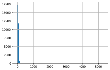 sns.boxplot(df_copy['full_sq'])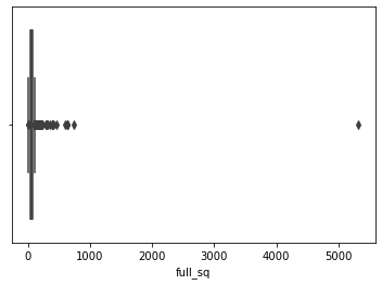 - Method #3: bar chart
# to check outliers in categorical attributes df['ecology'].value_counts().plot(kind='bar') # But if there is a category with only one value called ‘extraordinary’, that could be considered an ‘outlier’.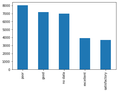 - How to handle missing data
- Unnecessary data
- Unnecessary type #1: repetitive & uninformative When an extremely high percentage of the column has a repetitive value,
num_rows = len(df_copy) for col in df_copy.columns: cnts = df_copy[col].value_counts(dropna=False) top_pct = (cnts/num_rows).iloc[0] if top_pct > 0.999: print('{0}: {1:.2f}%'.format(col, top_pct*100)) print(cnts) print()- Unnecessary type #2: irrelevant If features are not related to the question we are trying to solve, they are irrelevant. Use "drop()" method to drop such features
- Unnecessary type #3: duplicates
- duplicate occurs when all the columns’ values within the observations are the same.
df_copy[df_copy.duplicated()]id timestamp full_sq life_sq floor max_floor material build_year num_room kitch_sq ... cafe_count_5000_price_2500 cafe_count_5000_price_4000 cafe_count_5000_price_high big_church_count_5000 church_count_5000 mosque_count_5000 leisure_count_5000 sport_count_5000 market_count_5000 price_doc 0 rows × 292 columns
#We first drop id, and then see if there are duplicated rows from the DataFrame

df_copy[df_copy.drop(columns=['id']).duplicated()]
id timestamp full_sq life_sq floor max_floor material build_year num_room kitch_sq ... cafe_count_5000_price_2500 cafe_count_5000_price_4000 cafe_count_5000_price_high big_church_count_5000 church_count_5000 mosque_count_5000 leisure_count_5000 sport_count_5000 market_count_5000 price_doc 4328 4331 2012-10-22 61 -999.0 18.0 -999.0 -999.0 -999.0 -999.0 -999.0 ... 11 2 1 5 4 0 1 32 5 8248500 6991 6994 2013-04-03 42 -999.0 2.0 -999.0 -999.0 -999.0 -999.0 -999.0 ... 3 2 0 2 16 1 0 20 4 3444000 8059 8062 2013-05-22 68 -999.0 2.0 -999.0 -999.0 -999.0 -999.0 -999.0 ... 3 2 0 2 16 1 0 20 4 5406690 8653 8656 2013-06-24 40 -999.0 12.0 -999.0 -999.0 -999.0 -999.0 -999.0 ... 1 0 0 4 6 0 0 4 1 4112800 14004 14007 2014-01-22 46 28.0 1.0 9.0 1.0 1968.0 2.0 5.0 ... 10 1 0 13 15 1 1 61 4 3000000 17404 17407 2014-04-15 134 134.0 1.0 1.0 1.0 0.0 3.0 0.0 ... 0 0 0 0 1 0 0 0 0 5798496 26675 26678 2014-12-17 62 -999.0 9.0 17.0 1.0 -999.0 2.0 1.0 ... 371 141 26 150 249 2 105 203 13 6552000 28361 28364 2015-03-14 62 -999.0 2.0 17.0 1.0 -999.0 2.0 1.0 ... 371 141 26 150 249 2 105 203 13 6520500 28712 28715 2015-03-30 41 41.0 11.0 17.0 1.0 2016.0 1.0 41.0 ... 2 2 0 2 9 0 0 7 2 4114580 9 rows × 292 columns
(29779, 292) (29770, 291) # Inconsistent datadf_dedupped = df.drop(columns=['id']).drop_duplicates() print(df.shape) print(df_dedupped.shape)- Inconsistent type #1: capitalization Inconsistent use of upper and lower cases in categorical values is typical. We need to clean it since Python is case-sensitive.
Poselenie Sosenskoe 1617 Nekrasovka 1611 Poselenie Vnukovskoe 1290 Poselenie Moskovskij 925 Poselenie Voskresenskoe 713 Mitino 679 Tverskoe 678 Krjukovo 518 Mar'ino 508 Juzhnoe Butovo 451 Poselenie Shherbinka 443 Solncevo 421 Zapadnoe Degunino 410 Poselenie Desjonovskoe 362 Otradnoe 353 Nagatinskij Zaton 327 Nagornoe 305 Bogorodskoe 305 Strogino 301 Izmajlovo 300 Tekstil'shhiki 298 Ljublino 297 Gol'janovo 295 Severnoe Tushino 282 Chertanovo Juzhnoe 273 Birjulevo Vostochnoe 268 Vyhino-Zhulebino 264 Horoshevo-Mnevniki 262 Zjuzino 259 Ochakovo-Matveevskoe 255 Perovo 247 Ramenki 241 Jasenevo 237 Kosino-Uhtomskoe 237 Bibirevo 230 Golovinskoe 224 Poselenie Filimonkovskoe 221 Caricyno 220 Kuz'minki 220 Kon'kovo 220 Veshnjaki 213 Akademicheskoe 211 Orehovo-Borisovo Juzhnoe 208 Koptevo 207 Orehovo-Borisovo Severnoe 206 Novogireevo 201 Chertanovo Severnoe 200 Danilovskoe 199 Ivanovskoe 197 Mozhajskoe 197 Chertanovo Central'noe 196 Pechatniki 192 Presnenskoe 190 Sokolinaja Gora 188 Obruchevskoe 185 Kuncevo 184 Brateevo 182 Severnoe Butovo 182 Rjazanskij 180 Hovrino 178 Losinoostrovskoe 177 Juzhnoe Tushino 175 Dmitrovskoe 174 Taganskoe 173 Severnoe Medvedkovo 167 Beskudnikovskoe 166 Teplyj Stan 165 Pokrovskoe Streshnevo 164 Severnoe Izmajlovo 163 Cheremushki 158 Nagatino-Sadovniki 158 Troickij okrug 158 Shhukino 155 Timirjazevskoe 154 Vostochnoe Izmajlovo 154 Preobrazhenskoe 152 Novo-Peredelkino 149 Filevskij Park 148 Lomonosovskoe 147 Kotlovka 147 Juzhnoe Medvedkovo 143 Poselenie Pervomajskoe 142 Novokosino 139 Fili Davydkovo 137 Horoshevskoe 136 Levoberezhnoe 135 Donskoe 135 Vojkovskoe 131 Sviblovo 131 Zjablikovo 127 Troparevo-Nikulino 126 Lianozovo 126 Juzhnoportovoe 126 Ajeroport 123 Babushkinskoe 123 Jaroslavskoe 121 Lefortovo 119 Vostochnoe Degunino 118 Mar'ina Roshha 116 Birjulevo Zapadnoe 115 Matushkino 111 Savelki 105 Krylatskoe 103 Butyrskoe 101 Silino 100 Prospekt Vernadskogo 100 Alekseevskoe 100 Moskvorech'e-Saburovo 99 Basmannoe 98 Meshhanskoe 94 Staroe Krjukovo 92 Hamovniki 90 Savelovskoe 85 Marfino 85 Jakimanka 81 Ostankinskoe 79 Gagarinskoe 79 Nizhegorodskoe 77 Sokol 72 Altuf'evskoe 68 Rostokino 64 Kurkino 62 Sokol'niki 60 Begovoe 60 Metrogorodok 58 Dorogomilovo 56 Zamoskvorech'e 50 Kapotnja 49 Vnukovo 44 Krasnosel'skoe 37 Severnoe 37 Poselenie Rogovskoe 30 Poselenie Rjazanovskoe 26 Poselenie Kokoshkino 20 Poselenie Mosrentgen 19 Poselenie Krasnopahorskoe 19 Arbat 15 Vostochnoe 7 Poselenie Marushkinskoe 6 Molzhaninovskoe 3 Poselenie Voronovskoe 2 Name: sub_area, dtype: int64 ‘Poselenie Sosenskoe’ and ‘pOseleNie sosenskeo’ could refer to the same district.# to print full numpy array without ... #import numpy as np #import sys #np.set_printoptions(threshold=sys.maxsize) # to display the entire list without ... with pd.option_context('display.max_rows', None, 'display.max_columns', None): # more options can be specified also display(df_copy['sub_area'].value_counts(dropna=False))- How to handle? To avoid this, we can lowercase (or uppercase) all letters.
poselenie sosenskoe 1617 nekrasovka 1611 poselenie vnukovskoe 1290 poselenie moskovskij 925 poselenie voskresenskoe 713 ... arbat 15 vostochnoe 7 poselenie marushkinskoe 6 molzhaninovskoe 3 poselenie voronovskoe 2 Name: sub_area_lower, Length: 141, dtype: int64df_copy['sub_area_lower'] = df_copy['sub_area'].str.lower() df_copy['sub_area_lower'].value_counts(dropna=False)- Inconsistent type #2: typos of categorical values
A categorical column takes on a limited and usually fixed number of possible values. Sometimes it shows other values due to reasons like typos.
- We generate a new DataFrame, df_city_ex There is only one column that stores the city names. There are misspellings. For example, ‘torontoo’ and ‘tronto’ both refer to the city of ‘toronto’.
- The variable cities stores the 4 correct names of ‘toronto’, ‘vancouver’, ‘montreal’, and ‘calgary’.
- To identify typos, we use fuzzy logic matches. We use edit_distance from nltk, which measures the number of operations (e.g., substitution, insertion, deletion) needed to change from one string into another string.
- We calculate the distance between the actual values and the correct values.
vancouvr 1 montreal 1 vancover 1 turonto 1 calgary 1 vancouver 1 torontooo 1 toronto 1 Name: city, dtype: int64
# Levenshtein Distance, Hamming distance df_city_ex = pd.DataFrame(data={'city': ['torontooo', 'toronto', 'turonto', 'vancouver', 'vancover', 'vancouvr', 'montreal', 'calgary']}) df_city_ex['city'].value_counts()0 toronto 1 toronto 2 toronto 3 vancouver 4 vancouver 5 vancouver 6 montreal 7 calgary Name: city, dtype: object#!pip install pyspellchecker from spellchecker import SpellChecker spell = SpellChecker() i=0 for city in df_city_ex['city']: # Get the one `most likely` answer df_city_ex.at[i, 'city']= spell.correction(city) i=i+1 #print(spell.correction(city)) df_city_ex['city']vancouver 3 toronto 3 montreal 1 calgary 1 Name: city, dtype: int64 --- Tags: [!AMLIndex](./!AMLIndex.md)df_city_ex['city'].value_counts()
- How to find out?
Let’s see an example. Within the code below:
- Method #3: bar chart
- Method #1: descriptive statistics
- Method #2: missing data (by columns) heatmap